Wall posters
A home mountain, lake or city in one or two colors, printed large without pixelation.
Download contour lines as a true vector SVG: a free file with one path per line, or a layered SVG grouped by elevation in millimeters.
A .kml, .geojson or .json file with a Polygon or MultiPolygon, up to 5 MB. It is read in your browser and never uploaded. Samples: boulder-triangle.kml, test-parcel.geojson.
Every Nth contour is drawn bold (0 turns index lines off).
Terrain Tiles combine USGS 3DEP (about 10 m) in the US with SRTM and other 30 m data elsewhere, read on a 15 m grid (30 m above 100 km²).
Line colors follow elevation while Coloring is set to Elevation tints.
Contour interval 10 meters
Loading elevation for Boulder, CO…
Elevation: Terrain Tiles on AWS Open Data (USGS 3DEP, SRTM, GMTED2010 courtesy of the U.S. Geological Survey; ETOPO1 NOAA; and others) and, for Pro lidar, USGS 3DEP 1 m. Basemap, roads and place search © OpenStreetMap contributors (Nominatim). Full credits
Contours are generated from public elevation data. Accuracy depends on the source data, and they are not a substitute for a field survey or a licensed land survey.
The legend appears when the contours are ready.
Nothing saved yet. Saves stay in this browser only (localStorage).
Built on our server, in memory, from the contours on the map. Nothing is stored. Pricing
Layers appear when the contours are ready.
Groups appear when the contours are ready.
A folder per elevation, colored lines, labeled index lines and a legend overlay.
Zipped .shp, .shx, .dbf, .prj and .cpg with ELEV, UNIT and INDEX fields, in the coordinates chosen for DXF.
7357 × 8000 px
Add up to 20 areas, then download every chosen format for all of them in one zip, each area in its own folder in its local UTM zone.
Everything above the line stays free and unlimited. Pro adds CAD and print files, 1 m lidar for US sites, areas up to 2,000 km² and batches.
$9.99
One payment, every Pro feature for 7 days. No renewal.
$49 / year
Every Pro feature for a year. Renews yearly until you cancel.
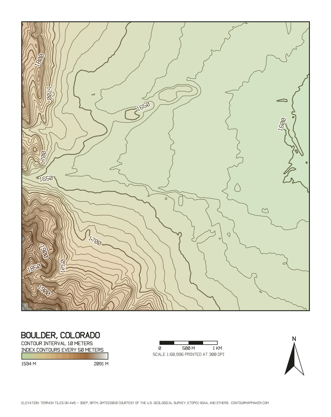
These previews come from the same contours the SVG exports write, rendered by the tool's own code at the settings shown. Open one to load the area, then download it as SVG.
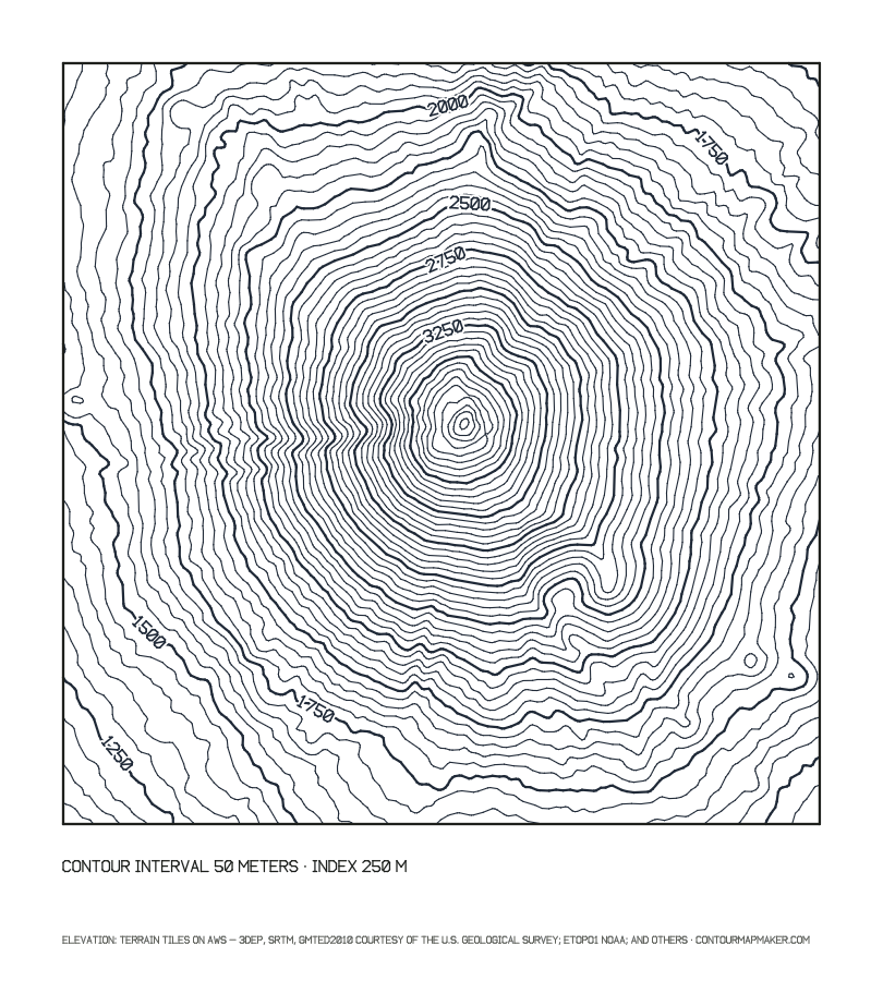
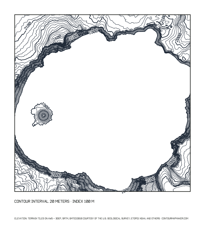
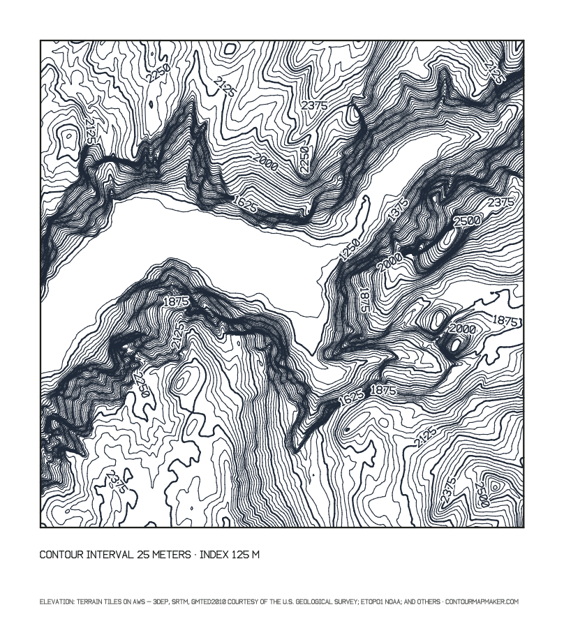
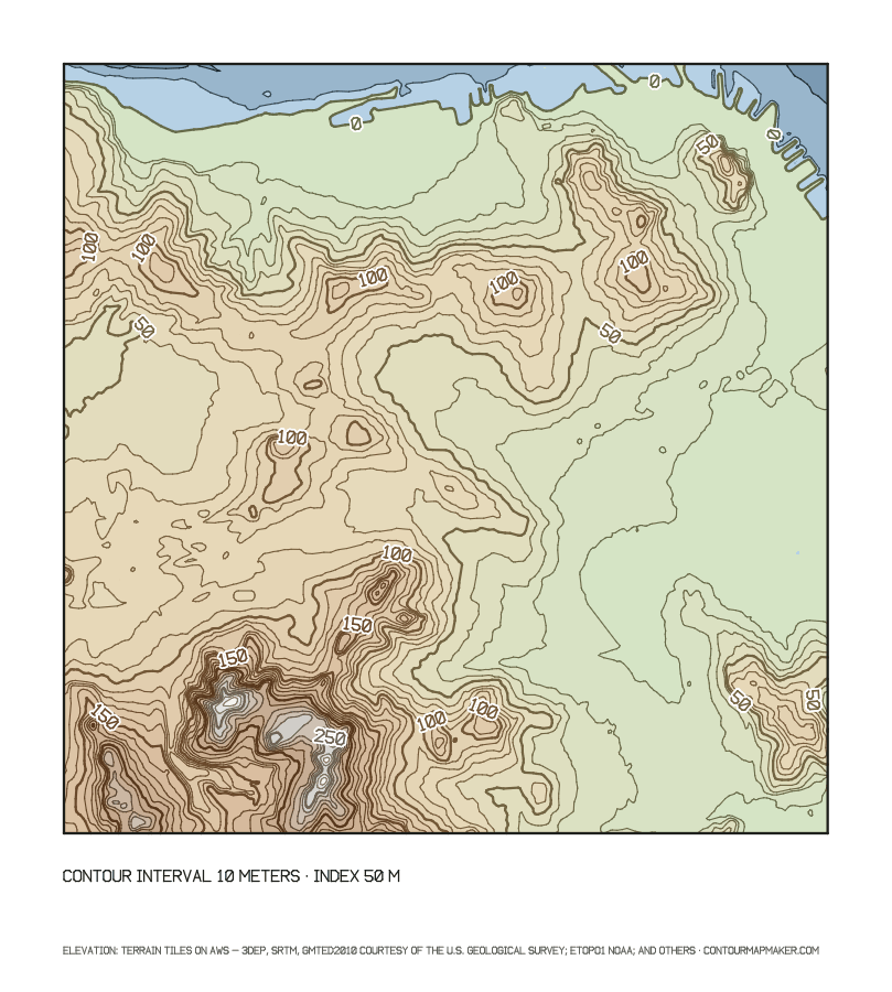
Both files are true vectors with one <path> per contour line, drawn in the same Web Mercator frame as the map so they line up with the PNG. The difference is structure. The basic SVG is a flat list of lines, which is all a poster or a quick Figma mockup needs. The layered SVG is organized for production work, where you want to select one elevation, hide labels or send a layer to a cutter.
| SVG (basic), free | Layered SVG, Pro | |
|---|---|---|
| Lines | One <path> per contour | One <path> per contour |
| Grouping | None | One <g id="elev-1600m"> per elevation, shown as layers in Inkscape |
| Index lines | Twice as thick | Twice as thick, labeled with the elevation |
| Labels | None | Separate labels group to engrave or hide |
| Size | Pixels, same frame as the 4096 px PNG | Millimeters at a stated scale; you set the sheet width |
| Line width | The width you set, in px | 0.25 mm × your width setting, index lines double |
| Credit | Comment in the file | Comment, description and a credits group |
Each elevation group in the layered SVG is one board. Cut the outline of that level and score the line of the next level on top of it, so you know where the next board sits when you glue the stack. With the Crater Lake example on a 420 mm sheet, the horizontal scale is about 1:21,429. At 20 m per 3 mm board, the vertical scale is 1:6,667, so the model is exaggerated 3.2 times vertically, which keeps a 600 m caldera wall readable on a desk. Thinner boards or a larger interval flatten it; a smaller area makes it steeper.
Two practical points. Lines that leave the area stay open at the frame, so close each board along the edge: draw the missing stretch of frame with the pen tool and join the end nodes. And small rings, such as a knoll a few boards high, produce tiny pieces; delete them or raise the interval.
For a poster, the free SVG at 40 to 60 levels gives the even line texture people expect. In Figma or Illustrator, set the stroke of everything at once, then pick out the index lines (class i in the file) and make them heavier. Put the title and coordinates in your own type. Keep the credit line somewhere on the print; the elevation data asks for it.
A home mountain, lake or city in one or two colors, printed large without pixelation.
Stacked plywood, acrylic or cardboard models with one board per elevation, from the layered SVG.
Subtle topographic textures for websites, apps and packaging, built from a real place rather than noise.
Single-line paths for pen plotters, engravers and embroidery software that need open strokes rather than fills.
An SVG for a poster wants 30 to 60 levels; a laser-cut model wants as many as you are willing to cut, usually 10 to 30. Find your area and relief below, then adjust toward the look you want.
| Area you select | Terrain | Relief | Interval, m | Interval, ft | Data that supports it |
|---|---|---|---|---|---|
| House lot or building site, under 0.1 km² (25 acres) | Gentle to hillside | 5–25 m | 0.5 | 1–2 | 3DEP 1 m lidar (Pro, US) for survey-grade lines; free data shows the shape |
| Small farm or acreage, 0.1–2 km² | Rolling | 20–100 m | 0.5–2 | 2–10 | 3DEP 1 m lidar (Pro, US) for survey-grade lines; free data shows the shape |
| Farm, ranch or park, 2–10 km² | Hilly | 100–300 m | 2–10 | 10–20 | 3DEP 1 m lidar (Pro, US) for survey-grade lines; free data shows the shape |
| Town or valley, 10–50 km² | Hills to foothills | 300–800 m | 10–20 | 20–80 | Free data in the US; elsewhere use 20 m or more |
| Mountain area, 50–100 km² (free limit) | Mountains | 800–2,000 m | 20–50 | 80–200 | Free data, worldwide |
| Range or region, 100–2,000 km² (Pro) | High mountains | 1,500–4,000 m | 50–100 | 100–500 | Free data, worldwide |
Relief is the highest minus the lowest elevation in your selection (the tool shows both under Map data). Interval = relief ÷ 50, rounded up to 0.5, 1, 2, 5, 10, 20, 25, 50, 100 or 200 m (1, 2, 5, 10, 20, 40, 50, 80, 100, 200, 250 or 500 ft). The last column applies the 1947 National Map Accuracy Standard, interval ≥ 3.29 × the data's vertical RMSE: about 0.3 m for lidar, 5.1 m for the US 10 m data and 18 m for SRTM.
Yes. Every contour line is its own <path> element with real coordinates, not an embedded picture, so it scales to any size and opens as editable lines in Figma, Illustrator, Inkscape, Affinity Designer and laser software. The Boulder sample at 10 m holds about 140 paths.
The free SVG has one path per line with no groups or labels, sized in pixels like the PNG. The Pro layered SVG puts every elevation in its own group (for example elev-1600m), which Inkscape shows as a layer, draws index lines twice as thick, keeps the elevation labels in a separate labels group, and is sized in millimeters at a stated scale.
Use the layered SVG. Each elevation group becomes one board: cut that level's line and score the next level up as a guide for gluing. Hide the labels group or set it to engrave. Lines that run off the edge of your area stay open, so close each layer along the frame in your editor, or choose an area where the lines close on themselves.
Drag the .svg file onto the Figma canvas, or open it in a text editor, copy everything and paste it into Figma. Figma keeps each path editable and turns the elevation groups of the layered SVG into groups in the layers panel, so you can recolor or hide whole elevations at once.
You choose the sheet width in millimeters, 420 mm by default, and the height follows the shape of your area. The scale is written in the file: a 9 km wide area on a 420 mm sheet is about 1:21,429. Line widths are 0.25 mm for intermediate contours and 0.5 mm for index contours at the default width of 1.
Yes. Both files style lines with a short CSS block at the top: change stroke-width there, or select a group in your editor and change its stroke. Index lines carry the class i, so you can restyle them separately.